A short note on Costa’s minimal surface

The other day, I finally managed to simplify Alfred Gray’s parametric equations for Costa’s minimal surface. I might edit this post later, with details on how to manipulate the Weierstrass elliptic functions that show up in the equations, but enjoy these for now:

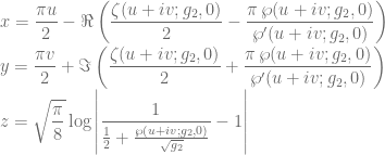
$\displaystyle x=\frac{\pi u}{2}-\Re\left(\frac{\zeta(u+iv;g_2,0)}{2}-\frac{\pi\,\wp(u+iv;g_2,0)}{\wp^\prime(u+iv;g_2,0)}\right) \\ y=\frac{\pi v}{2}+\Im\left(\frac{\zeta(u+iv;g_2,0)}{2}+\frac{\pi\,\wp(u+iv;g_2,0)}{\wp^\prime(u+iv;g_2,0)}\right) \\ z=\sqrt{\frac{\pi}{8}}\log\left|\frac1{\frac12+\frac{\wp(u+iv;g_2,0)}{\sqrt{g_2}}}-1\right|$

Here, $\wp, \wp^\prime$ and $\zeta$ are respectively the Weierstrass elliptic function, its derivative, and the Weierstrass zeta function, with invariants $g_2=\left(\frac12\mathrm{B}\left(\frac14,\frac14\right)\right)^4=\frac{\Gamma(1/4)^8}{16\pi^2}$ and $0$ , and $\mathrm{B}(x,y)$ and $\Gamma(x)$ are the usual beta and gamma functions. The invariants are the ones corresponding to the semi-periods $\omega_1=\frac12$ and $\omega_3=\frac{i}{2}$ . The parameter ranges are $0 < u < 1$ and $0 < v < 1$ .

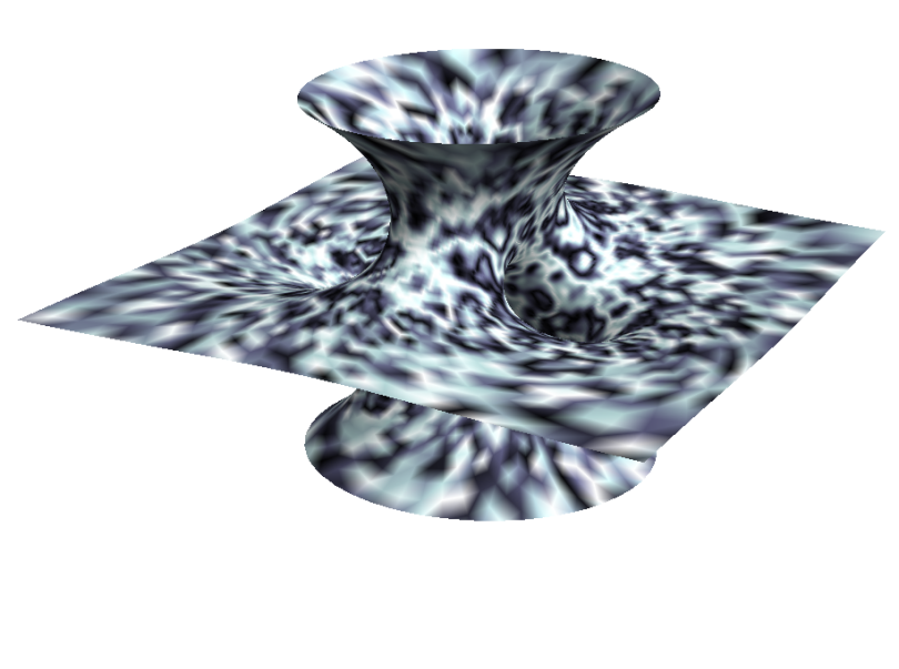
I was very delighted at my result, that I decided to make a stylized plot of the surface in Mathematica, using Perlin’s simplex noise for the coloring: