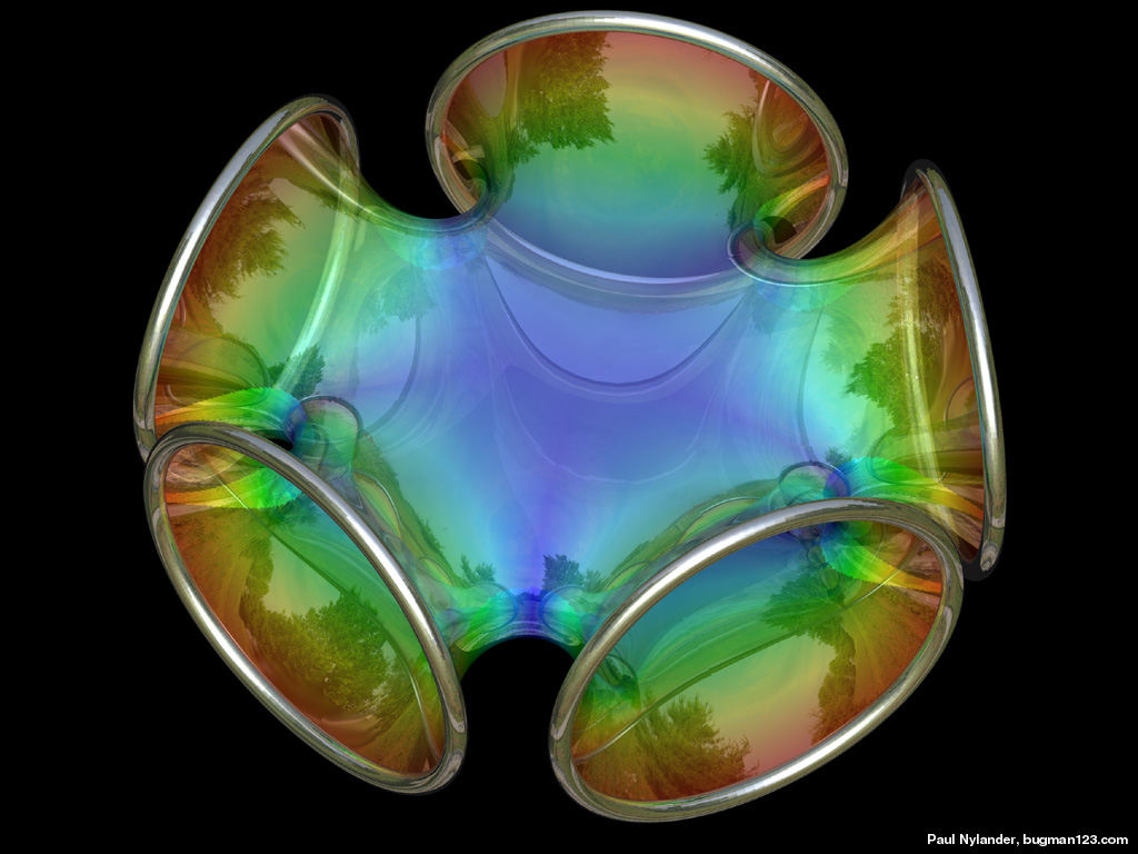
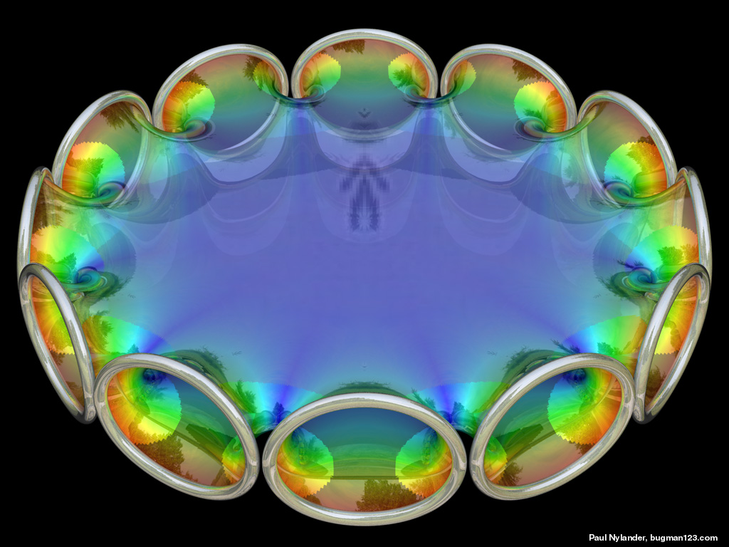
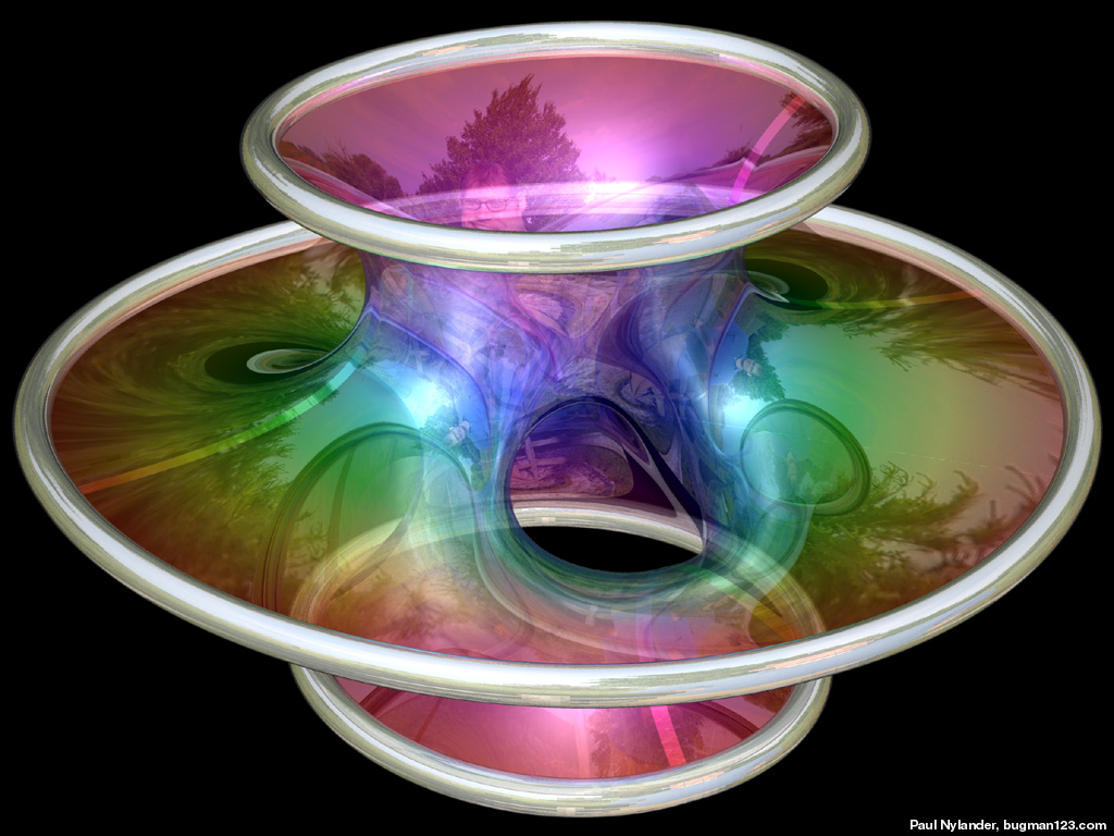
 The Chen-Gackstatter Minimal Surface is a modified Enneper surface with holes in it. The following Mathematica code uses some functions that were adapted from Matthias Weber’sMathematica notebook:
(* runtime: 0.4 second *)

<< Graphics`Shapes`; k = 5; n = (k - 1)/k; rho = 1.0/Sqrt[4^n Gamma[(3 - n)/2] Gamma[1 + n/2]/(Gamma[(3 +n)/2]Gamma[1 - n/2])];

phi[n_, z_] := z^(1 + n)Hypergeometric2F1[(1 + n)/2, n, (3 + n)/2, z^2]/(1 + n); f[z_] := {0.5(phi[n, z]/rho - rho phi[-n, z]), 0.5I(rho phi[-n, z] + phi[n, z]/rho), z};

surface = ParametricPlot3D[Re[f[r Exp[I theta]]], {r, 0, 2}, {theta, 1*^-6, 2Pi}, PlotPoints -> {9, 33}, Compiled -> False, DisplayFunction -> Identity][[1]];

Show[Graphics3D[Table[RotateShape[surface, 0, 0, 2Pi i/k], {i, 0, k - 1}]]]
Archive for the 'Minimal surfaces' Category
Chen-Gackstatter Minimal Surface
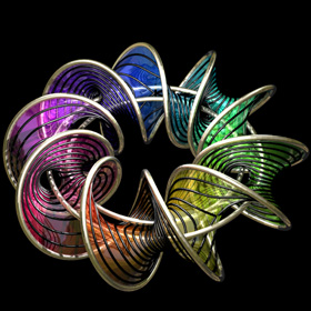
Scherk-Collins Surface
 This surface can be formed by twisting and warping a singly-periodic Scherk’s minimal surface. This idea was originally attributed to Brent Collins. Technically, the surface is no longer considered exactly “minimal” after twisting but it still looks minimal (it is actually very difficult to find the exact shape for most minimal surfaces). Click here to download some POV-Ray code.
Here is some Mathematica code:
(* runtime: 0.3 second *)

<< Graphics`Master`; n = 5; r = 0.75n;

Twist[{x_, y_, z_}, theta_] := {x Cos[theta] - y Sin[theta], x Sin[theta] + y Cos[theta], z};

Warp[{x_, y_, z_}, theta_] := {(x + r) Cos[theta], (x + r) Sin[theta], y};

f[z_] := Module[{t1 = Sqrt[2Cot[z]], t2 = Cot[z] + 1}, Warp[Twist[Re[{0.5xsign(Log[t1 - t2] - Log[t1 + t2])/Sqrt[2], ysign I(ArcTan[1 - t1] - ArcTan[1 + t1])/Sqrt[2], z}], 2Re[z]/n], 2Re[z]/n]];

DisplayTogether[Table[ParametricPlot3D[f[x + I y], {x, 0, n Pi}, {y, 0.001, 0.75}, PlotPoints -> {8n + 1, 5}, Compiled -> False], {xsign, -1, 1, 2}, {ysign, -1, 1, 2}]]
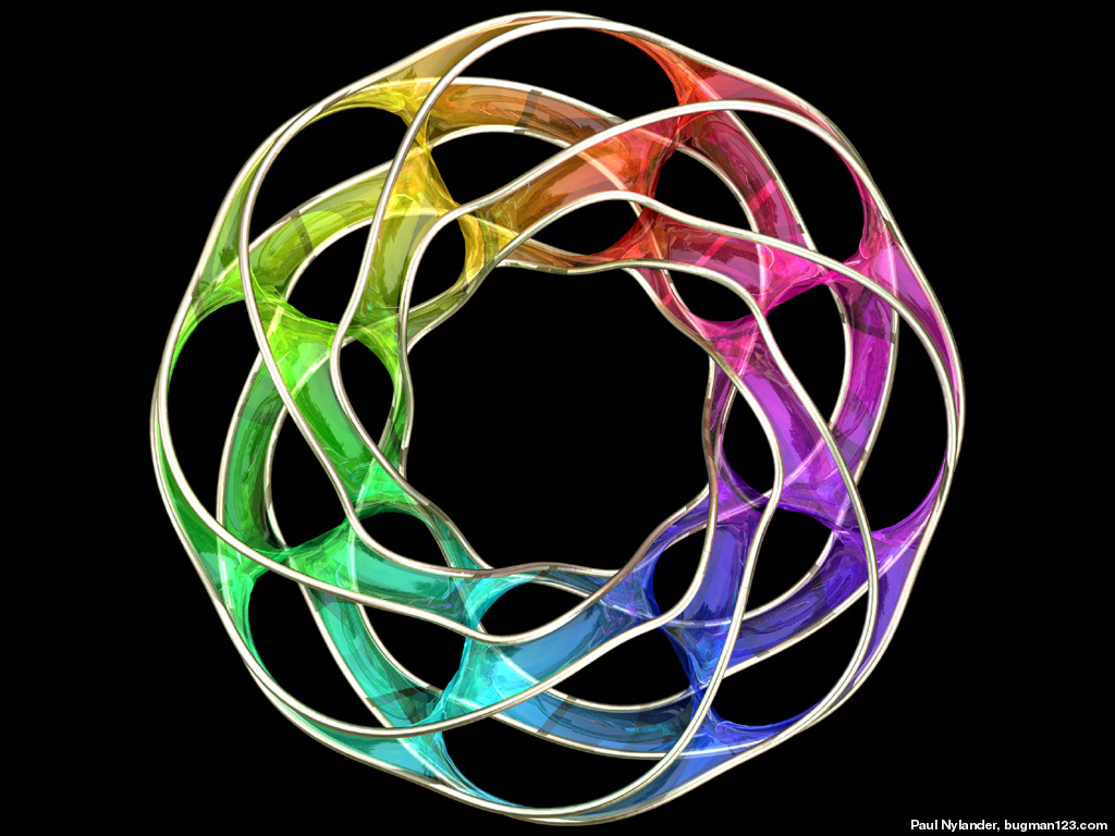
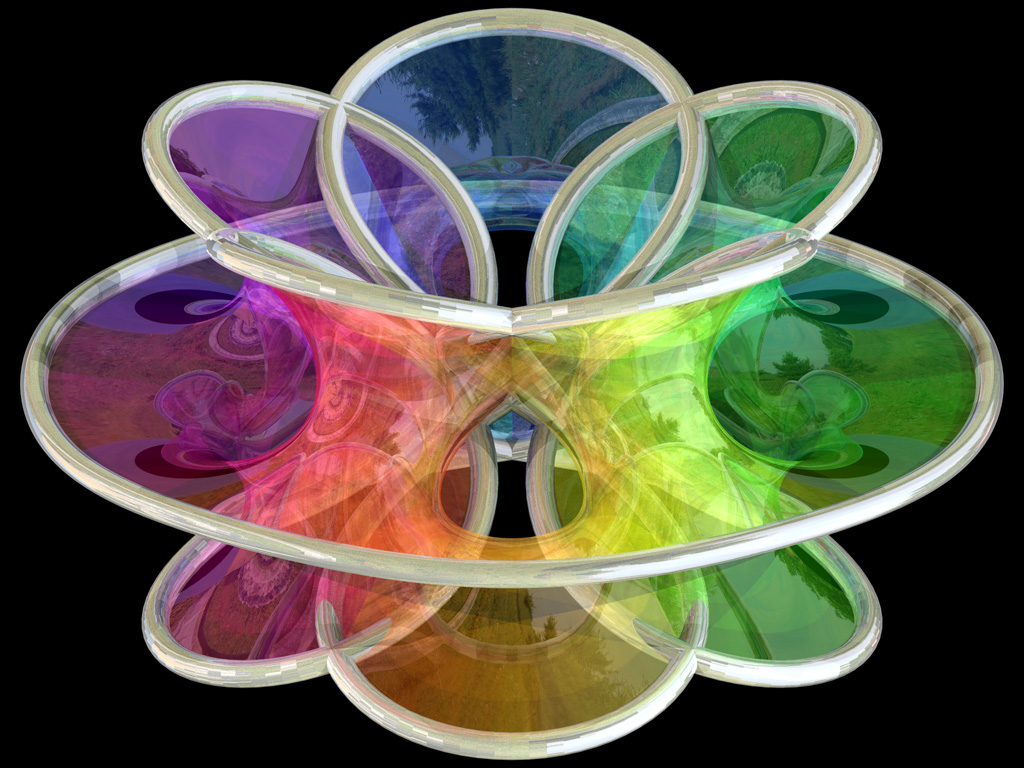
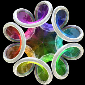
The following Mathematica code can be used to increase the number of edges (or “branches”). This code uses some complicated functions that were adapted from Matthias Weber’s Mathematica notebook:
(* runtime: 1.2 seconds *)

<< Graphics`Shapes`; k = 4; phi = Pi(0.6/k - 0.5)/(1 - k);

f[z_] := Re[NIntegrate[Evaluate[{0.5 (w^(1 - k) - w^(k - 1)), 0.5 I (w^(1 - k) + w^(k - 1)), 1}/(w^(k + 1) + w^(1 - k) - 2w Cos[k phi])], {w, 0, z}]];

alpha = Pi/k; zbeta = Exp[I Pi(phi/alpha - 0.5)];

surface = ParametricPlot3D[Re[f[Exp[I alpha/2]((1 + I zbeta Exp[r + I theta])/(I Exp[r + I theta] -zbeta))^(alpha/Pi)]], {r, 0, 4}, {theta, 0, Pi}, PlotPoints -> 10, Compiled -> False, DisplayFunction -> Identity][[1]];

z0 = f[1][[3]]; surface = {surface, AffineShape[TranslateShape[surface, {0, 0, -2z0}], {1, 1, -1}]};

surface = {surface, AffineShape[surface, {1, -1, 1}]}; surface = Table[RotateShape[surface, 2Pi i/k, 0, 0], {i, 1, k}];

dz = Pi Csc[k phi]/k; Show[Graphics3D[Table[TranslateShape[surface, {0, 0, i dz}], {i, 0, 1}]]]
Links
- “Whirled White Web” – a beautiful snow sculpture by Brent Collins
- Sculpture Generator – C++ program for Scherk-Collins surfaces by Carlo Séquin
- Bathsheba Grossman – metal printed math sculptures
- Torolf Sauermann – math art
Punctured Helicoid

 Here is a helicoidwith holes in it. The following Mathematica code uses some complicated functions that were adapted from Matthias Weber’sMathematica notebook:
(* runtime: 4 seconds *)

<< Graphics`Shapes`;

tau0 = Exp[1.23409 I]; b0 = 0.629065; theta[z_] := EllipticTheta[1, Pi z, Exp[I Pi tau0]];

r1[z_] := theta[z + 0.5 (b0 - 2) (tau0 + 1)]/theta[z + 0.5 (b0 - 1) (tau0 + 1)]; r2[z_] := theta[z - 0.5 b0 (tau0 + 1)]/theta[z - 0.5 (b0 + 1) (tau0 + 1)];

omega3[z_] := r1[z] r2[z]/(0.386191 - 0.169839 I); G[z_] := (108.37 - 62.8417 I) Exp[I Pi (b0 - 2 z + 2 tau0 + b0 tau0)]r1[z]/r2[z];

f[z0_] := Re[NIntegrate[Evaluate[{-(G[z] omega3[z] - omega3[z]/G[z] )/2, I(G[z] omega3[z] + omega3[z]/G[z] )/2, omega3[z]}], {z, tau0/2, z0}]] + {0.434156, 0, -1};

a0 = -0.409956; r0 = 2.43051; g[z_] := (EllipticF[ArcSin[(a0 + r0 E^z)/(1 - a0 E^z)], 1/r0^2]/(2EllipticF[Pi/2, 1/r0^2]) + 0.5)(1 + tau0)/2;

surface = ParametricPlot3D[f[g[x + I y]], {x, -2.5, 2.5 - 0.8881}, {y, 0.001,0.999Pi}, PlotPoints -> {15, 10}, Compiled -> False, DisplayFunction -> Identity][[1]];

surface = {surface, RotateShape[surface, 0, 0, Pi]};

Show[Graphics3D[{surface, TranslateShape[surface, {0, 0, 2}]}, ViewPoint -> {1, 6, 3}]];
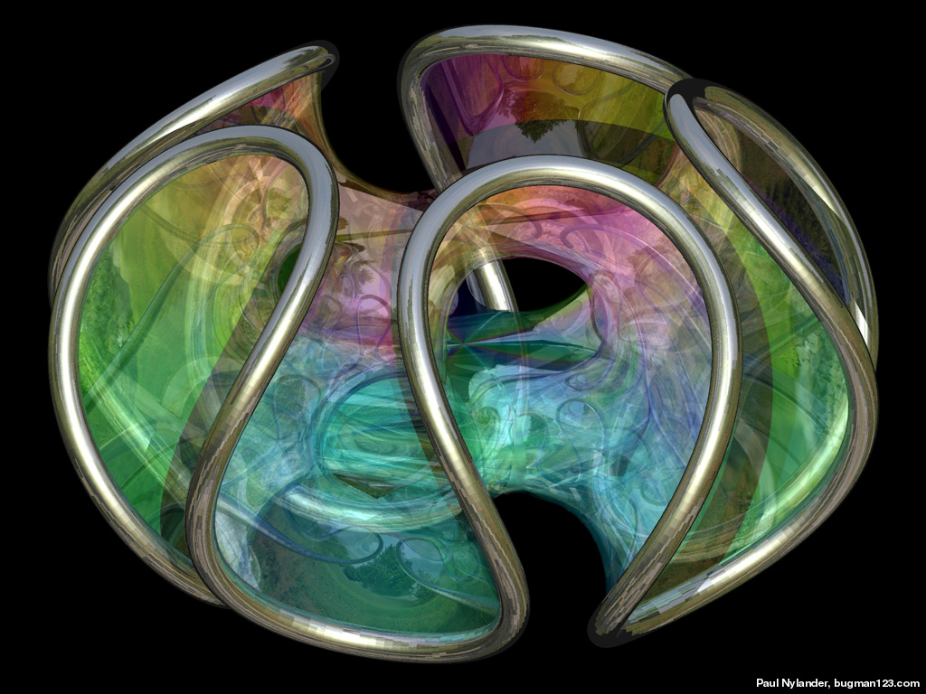
Jorge-Meeks K-Noids
The following Mathematica code uses some functions that were adapted from Matthias Weber’sMathematica notebook:
(* runtime: 0.4 second *)

<< Graphics`Shapes`;

k = 5; phi1[z_] := z^(k - 1) (k/(1 - z^k) - (k - 1) LerchPhi[z^k, 1, 1 - 1/k])/k^2; phi2[z_] := z(1/(1 - z^k) + (k - 1)LerchPhi[z^k, 1, 1/k]/k)/k;

f[z_] := {0.5 (phi2[z] - phi1[z]), 0.5 I (phi1[z] + phi2[z]), 1/(k - k z^k)};

surface = ParametricPlot3D[Re[f[(1 + 2/(I Exp[x + I y] - 1))^(2/k)]], {x,0, Pi/2}, {y, -Pi/2, Pi/2}, PlotPoints -> {8, 16}, Compiled -> False, DisplayFunction -> Identity][[1]];

surface = {surface, AffineShape[surface, {1, -1, 1}]};

Show[Graphics3D[Table[RotateShape[surface, 0, 0, 2Pi i/k], {i, 0, k - 1}]]];
Links
Catenoid/Helicoid


 This minimal surface is a cross between acatenoid andhelicoid. It would be interesting to see what really happens when a spring is covered with a soap film. Click here to download some POV-Ray code. Here is some Mathematica code:
(* runtime: 0.6 second *)

x := Sin[alpha]Cosh[v]; y := Cos[alpha]Sinh[v];

Do[ParametricPlot3D[{x Cos[u] + y Sin[u], x Sin[u] - y Cos[u], u Cos[alpha] + v Sin[alpha]}, {u, 0, 2Pi}, {v, -2.25, 2.25}, PlotPoints -> {36, 10}], {alpha, -Pi/2, Pi/2, Pi/18}];
Links
- Venice Museum Bridge – bridge proposal, by Eric Worcester
- Marina Bayfront Pedestrian Bridge – double-helix bridge in Singapore
- Soap Film Coil Photo – by the Exploratorium
Richmond’s Minimal Surface
 I learned about this minimal surface from Brian Johnston’s website. Here is some Mathematica code:
(* runtime: 2 seconds *)

Richmond[n_, z_] := {-1/(2z) - z^(2n + 1)/(4n + 2), -I/(2z) + I z^(2n + 1)/(4n + 2), z^n/n};

ParametricPlot3D[Re[Richmond[5, r Exp[I theta]]], {r, 0.53, 1.187}, {theta, 0, 2Pi}, PlotPoints -> {25, 180}, Compiled -> False]
Fourth Enneper Surface
 Click here to download some POV-Ray code for this image.
Here is some Mathematica code for the Second Enneper Surface:
(* runtime: 0.5 second *)

n = 3; ParametricPlot3D[{r Cos[phi] - r^(2n - 1) Cos[(2n - 1) phi]/(2n - 1), r Sin[phi] + r^(2n - 1) Sin[(2n - 1) phi]/(2n - 1), 2 r^n Cos[n phi]/n, EdgeForm[]}, {phi, 0, 2Pi}, {r, 0, 1.3}, PlotPoints -> {181, 20}, ViewPoint -> {0, 0, 1}, PlotRange -> All]
Link : Enneper Mathematica
Costa’s Minimal Surface
 Costa’s Minimal Surface is a classic example of a minimal surface with holes in it, also called “handles”. The number of holes is called the genus of the surface. This surface was discovered by a graduate student. I think it would be interesting to see someone create an actual soap film with this shape.
Here is some Mathematica code:
(* runtime: 5 seconds *)

c = 189.07272; e1 = 6.87519;

Costa[u_, v_] := Module[{z =u + I v}, zeta = WeierstrassZeta[z, {c, 0}]; zeta1 = WeierstrassZeta[z - 1/2, {c, 0}]; zeta2 = WeierstrassZeta[z - I/2, {c, 0}]; p = WeierstrassP[z, {c, 0}]; x = Re[Pi (u + Pi/(4 e1) ) - zeta + Pi(zeta1 - zeta2)/(2 e1)]/2; y = Re[Pi (v + Pi/(4 e1)) - I(zeta + Pi(zeta1 - zeta2)/(2 e1))]/2; z = (Sqrt[2 Pi]/4)Log[Abs[(p - e1)/(p + e1)]]; {x, y, z, EdgeForm[]}];

ParametricPlot3D[Costa[u, v], {u, 0.0001, 1}, {v, 0.0001, 1}, PlotPoints -> 40, PlotRange -> {{-3.5, 3.5}, {-3.5, 3.5}, {-2, 2}},Compiled -> False]
Here is another parametrization:
(* runtime: 5 seconds *)

Costa[z_] := Module[{phi1 = -2 Sqrt[z] Sqrt[1 - z^2] Hypergeometric2F1[1/4, 3/2, 5/4, z^2]/Sqrt[z^2 - 1], phi2 = -(2/3) z^(3/2) Sqrt[z^2 - 1] Hypergeometric2F1[3/4, 1/2, 7/4, z^2]/Sqrt[1 - z^2]}, Re[{phi2 - phi1, I(phi1 +phi2), Log[z - 1] - Log[z + 1]}]/2];

surface = ParametricPlot3D[Costa[Sqrt[Exp[r - I theta] + 1]], {r, -3.5, 6}, {theta, -Pi, Pi}, PlotPoints -> {20, 18}, Compiled -> False][[1]];

<< Graphics`Shapes`; surface = {surface, RotateShape[surface, Pi, 0, 0]}; Show[Graphics3D[{surface, RotateShape[surface, Pi/2, Pi, 0]}]]
Links
- Mathematica code and minimal surface art – by Matthias Weber
- Alfred Gray – differential geometry gallery
- soap bubble light interference – by Kei Iwasaki
- Eva Hild – beautiful ceramic sculptures
- minimal surfaces with metal frames
- Helaman Ferguson – math sculptor, see his Costa snow sculpture
 RSS feed
Recent Comments